Getting Started
This section walks you through a brief introduction to using IAMReX.
Downloading the code
IAMReX is built on top of the AMReX framework. In order to run IAMReX, you must download separate git modules for IAMReX, AMReX and AMReX-Hydro.
First, make sure that git is installed on your machine.
Download the AMReX repository by typing:
git clone https://github.com/ruohai0925/amrex.git
This will create a folder called
amrex/on your machine.Download the AMReX-Hydro repository by typing:
git clone https://github.com/ruohai0925/AMReX-Hydro.git
This will create a folder called
AMReX-Hydro/on your machine.Download the IAMReX repository by typing:
git clone https://github.com/ruohai0925/IAMReX.git
This will create a folder called
IAMReX/on your machine.
After cloning, one will have three folders in your current directory: AMReX, AMReX-Hydro, IAMReX.
Note
Note that we use forked versions of the AMReX repository and AMReX-Hydro. The main reason for this is that we do not want upstream features to influence our downstream application codes. Considering we do not have sufficient computational resources to run nightly regression tests every day, it is better for us to maintain our own control over the specific versions of AMReX and AMReX-Hydro that IAMReX depends on.
Building the code
We recommend using the GNU compiler to compile the program on the Linux platform. The compilation process requires preparing a make file, which you can find in the example folder under Tutorials. It is strongly recommended to use the GNUmakefile prepared in advance by the example. If you want to know more about the configuration information of the compilation parameters, you can check it in the AMReX building.
For example, if we want to compile in the FlowPastSphere, refer to the following steps:
cd to the FlowPastSphere directory
cd IAMReX/Tutorials/FlowPastSphere
Modify compilation parameters in GNUmakefile.
The compilation parameters depend on your computing platform. AMReX uses an MPI+X strategy, where MPI distributes work across nodes (and GPUs), and X is a node-level parallelization backend—on GPUs, this is typically CUDA
- Use the following flags:
USE_MPI=TRUE to enable MPI
USE_CUDA=TRUE to enable CUDA
CUDA_ARCH=XX to specify the CUDA architecture (e.g., 80 for Ampere)
For more information on setting up MPI and CUDA environments, please refer to: OpenMPI, MPICH, IntelMPI, and CUDA.
Compile
With the above settings, you can compile the program:
make
You can add parameters after make, such as -f your_make_file to customize your parameter file, and -j 8 to specify 8 threads to participate in the compilation.
If the compilation is successful, an executable file will be generated. Usually the executable file is named in the following format:amr[DIM].[Compiler manufacturers].[computing platform].[is Debug].ex. The executable file name of the Release version of the three-dimensional compiled using the GNU compiler in the MPI environment is: amr3d.GNU.MPI.ex.
Running the code
You should take an input file as its first command-line argument. The file may contain a set of parameter definitions that will overrides defaults set in the code. In the FlowPastSphere, you can find a file named inputs.3d.flow_past_sphere, run:
./amr3d.GNU.MPI.ex inputs.3d.flow_past_sphere
If you use MPI to run your program, you can type:
mpirun -np how_many_processes amr3d.GNU.MPI.ex inputs.3d.flow_past_sphere
This code typically generates subfolders in the current folder that are named plt00000, plt00010, etc, and chk00000, chk00010, etc. These are called plotfiles and checkpoint files. The plotfiles are used for visualization of derived fields; the checkpoint files are used for restarting the code.
Visualization
Various tools are available for data postprocessing and visualization, one can check AMReX for reference. As for the specific settings and output content, IAMR also provides more details.
Since IAMReX uses the native plotfile format, the particle data is generated as CSV files in the same case directory following the naming convention IB_Particle_<ID>.csv
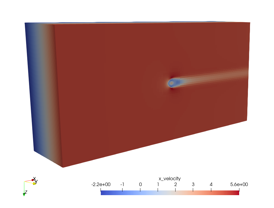
Figure 5 To visualize plotfiles, use ParaView to process and display the results.
The plotfiles include the quantities of several simulation parameters as output (density, gradpx, gradpy, gradpz, x_velocity, y_velocity, z_velocity and tracer).
Furthermore, particle data processing scripts are provided herein IBParticle2VTK. These utilities enable conversion of particle CSV files to VTK format, facilitating further analysis in ParaView.
Key parameters
Tip
One can also find more parameters in the IAMR guide.
Description |
Type |
Default |
|
|---|---|---|---|
do_diffused_ib |
enable IBM |
Int |
0 |
fluid_rho |
density of fluid |
Real |
1.0 |
The above parameters are designed for the immersed boundary (IB) method. Additionally, the particle.input flag (such as particle_inputs) must be specified to define IB-related parameters. The program will query these parameters through this flag. The specific parameters include the following:
Description |
Type |
Default |
|
|---|---|---|---|
x |
particle x position |
Real Array |
0.0 |
y |
particle y position |
Real Array |
0.0 |
z |
particle z position |
Real Array |
0.0 |
rho |
density of particles |
Real Array |
1.0 |
radius |
radius of particles |
Real Array |
0.0 |
velocity_x |
The initial velocity of the particles in the x direction |
Real Array |
0.0 |
velocity_y |
The initial velocity of the particles in the y direction |
Real Array |
0.0 |
velocity_z |
The initial velocity of the particles in the z direction |
Real Array |
0.0 |
omega_x |
The initial angular velocity of the particle around the x-axis |
Real Array |
0.0 |
omega_y |
The initial angular velocity of the particle around the y-axis |
Real Array |
0.0 |
omega_z |
The initial angular velocity of the particle around the z-axis |
Real Array |
0.0 |
TLX |
Particle freedom in x-direction |
Int Array |
0 |
TLY |
Particle freedom in y-direction |
Int Array |
0 |
TLZ |
Particle freedom in z-direction |
Int Array |
0 |
RLX |
Particle rotation about x-axis |
Int Array |
0 |
RLY |
Particle rotation about y-axis |
Int Array |
0 |
RLZ |
Particle rotation about z-axis |
Int Array |
0 |
RD |
particle retraction distance |
Real |
0.0 |
write_freq |
How many steps to export the particle information |
Int |
1 |
LOOP_NS |
Ns loop time |
Int |
2 |
LOOP_SOLID |
particle update steps |
Int |
1 |
start_step |
How much steps does it take for the particles to move |
Int |
-1 |
collision_model |
particle collision model |
Int |
1.0 |
verbose |
Whether to output debug information |
Int |
0 |
init |
particle init file path |
file path |
Checkpoints are used to resume simulations. You typically need to specify how often to save checkpoint files. To restart a simulation from a particular checkpoint, you must specify it in the restart parameters. These settings are usually defined under the amr field.
# how many timestep frequency to save checkpoint files
amr.check_int = 4000
# which checkpoint file to restart
amr.restart = chk00010
Among above parameters, array-type parameters are used to specify parameters for multiple particles individually, or define particle positions via an init file (e.g., a precomputed position data file). If particle positions are provided through an external file, other array-type parameters only need to provide a single value, which will be applied to all particles uniformly.
Example inputs file:
#*******************************************************************************
# INPUTS.3D.FLOW_PAST_SPHERE
#*******************************************************************************

#NOTE: You may set *either* max_step or stop_time, or you may set them both.

# Maximum number of coarse grid timesteps to be taken, if stop_time is
#  not reached first.
max_step         = 2

# Time at which calculation stops, if max_step is not reached first.
stop_time         = 100.0

ns.fixed_dt     = 0.01
ns.cfl = 0.3
ns.init_iter = 0

# Diffused IB input file
particle.input = particle_inputs

# Refinement criterion, use vorticity and presence of tracer
amr.refinement_indicators = tracer

amr.max_level        = 0 # maximum number of levels of refinement
# amr.tracer.value_greater = 0.1
# amr.tracer.value_less = 1.1
amr.tracer.field_name = tracer
amr.tracer.in_box_lo = 0.5 0.5 0.5
amr.tracer.in_box_hi = 1.5 1.5 1.5

amr.blocking_factor     = 8

#*******************************************************************************

# Number of cells in each coordinate direction at the coarsest level
# amr.n_cell         = 16 8 8
amr.n_cell         = 256 128 128
# amr.n_cell         = 288 128 128
amr.max_grid_size    = 16
# amr.max_grid_size    = 32

#*******************************************************************************

# Interval (in number of level l timesteps) between regridding
amr.regrid_int        = 1 # regrid_int

#*******************************************************************************

# Refinement ratio as a function of level
amr.ref_ratio        = 2 2 2 2

#*******************************************************************************

# Sets the "NavierStokes" code to be verbose
ns.v                    = 1
nodal_proj.verbose      = 1
mac_proj.verbose        = 1

# mac_proj.mac_tol        = 0.1
# mac_proj.mac_abs_tol    = 0.1

#*******************************************************************************

# Sets the "amr" code to be verbose
amr.v                   = 1

#*******************************************************************************

# Interval (in number of coarse timesteps) between checkpoint(restart) files

amr.check_int        = 4000

#amr.restart             = chk01400

#*******************************************************************************

# Interval (in number of coarse timesteps) between plot files
amr.plot_int        = 1


#*******************************************************************************

# Viscosity coefficient
ns.vel_visc_coef        = 0.01

#*******************************************************************************

# Diffusion coefficient for first scalar
ns.scal_diff_coefs      = 0.0

#*******************************************************************************

# Forcing term defaults to  rho * abs(gravity) "down"
ns.gravity              = 0.0 # -9.8

#*******************************************************************************

# skip level_projector
ns.skip_level_projector = 0

#*******************************************************************************

# subcycling vs. non-subcycling
amr.subcycling_mode     = None

#*******************************************************************************

# Set to 0 if x-y coordinate system, set to 1 if r-z.
geometry.coord_sys   =  0

#*******************************************************************************

# Physical dimensions of the low end of the domain.
geometry.prob_lo     =  0. 0. 0.

# Physical dimensions of the high end of the domain.
geometry.prob_hi     =  20. 10. 10.

#*******************************************************************************

#Set to 1 if periodic in that direction
geometry.is_periodic =  0 1 1

#*******************************************************************************

# Boundary conditions on the low end of the domain.
ns.lo_bc             = 1 0 0

# Boundary conditions on the high end of the domain.
ns.hi_bc             = 2 0 0

# 0 = Interior/Periodic  3 = Symmetry
# 1 = Inflow             4 = SlipWall
# 2 = Outflow            5 = NoSlipWall

# Boundary condition
xlo.velocity            =   1.  0.  0.

#*******************************************************************************

# Problem parameters
prob.probtype = 1

#*******************************************************************************

# Add vorticity to the variables in the plot files.
# amr.derive_plot_vars    = avg_pressure

#*******************************************************************************
ns.isolver            = 1
ns.do_diffused_ib     = 1
ns.fluid_rho          = 1.0

#ns.sum_interval       = 1

particles.do_nspc_particles = 0

nodal_proj.proj_tol = 1.e-8
nodal_proj.proj_abs_tol = 1.e-9

nodal_proj.maxiter = 200
nodal_proj.bottom_maxiter = 200

mac_proj.mac_tol = 1.e-8
mac_proj.mac_abs_tol = 1.e-9


############################
#                          #
#  Diffused IB cfg file    #
#                          #
############################

# particle's location
# x = p1x p2x p3x ...
particle_inputs.x = 5.0
particle_inputs.y = 5.0
particle_inputs.z = 5.0

# particle's density
# rho = p1r p2r p3r ...
particle_inputs.rho = 1.0

# particle's radius
# single
particle_inputs.radius = 0.5

# particle's velocity
# vx = p1vx p2vx p3vx ...
particle_inputs.velocity_x = 0.0
particle_inputs.velocity_y = 0.0
particle_inputs.velocity_z = 0.0

# particle's omega
# omega = p1omega_x p2omega_x p3omega_x ...
particle_inputs.omega_x = 0.0
particle_inputs.omega_y = 0.0
particle_inputs.omega_z = 0.0

# particle's 6DOF
# TLX = p1tl p2tl ...
particle_inputs.TLX = 0
particle_inputs.TLY = 0
particle_inputs.TLZ = 0
particle_inputs.RLX = 0
particle_inputs.RLY = 0
particle_inputs.RLZ = 0


# msg print
particle_inputs.verbose = 1
If you want to know more about the parameters, you can check the AMReX.
Tests
Test_IAMReX is a customized python script to evaluate the codebase’s structural completeness and to verify the accuracy of its computational results. A set of representative benchmark cases has been included, such as lid-driven cavity, RSV, Drafting–Kissing–Tumbling, flow past a cylinder, flow past a sphere, and Rayleigh–Taylor instability. These cases collectively assess a wide range of physical scenarios and computational modules. Furthermore, users may extend the testing framework by following the provided examples to construct additional test cases as needed.
Meanwhile, a continuous integration pipeline has been established using GitHub Actions to automate the execution and validation of these tests. The GitHub action only support 2 CPU cores, and GPU is not supported.
During the code development process, we have made every effort to ensure consistency between GPU and CPU results for each test case. For instance, in the Flow Past Sphere case, we conducted simulations at various Reynolds numbers to compare drag coefficients under both CPU and GPU execution modes, with and without adaptive mesh refinement (AMR). The corresponding results are presented below.
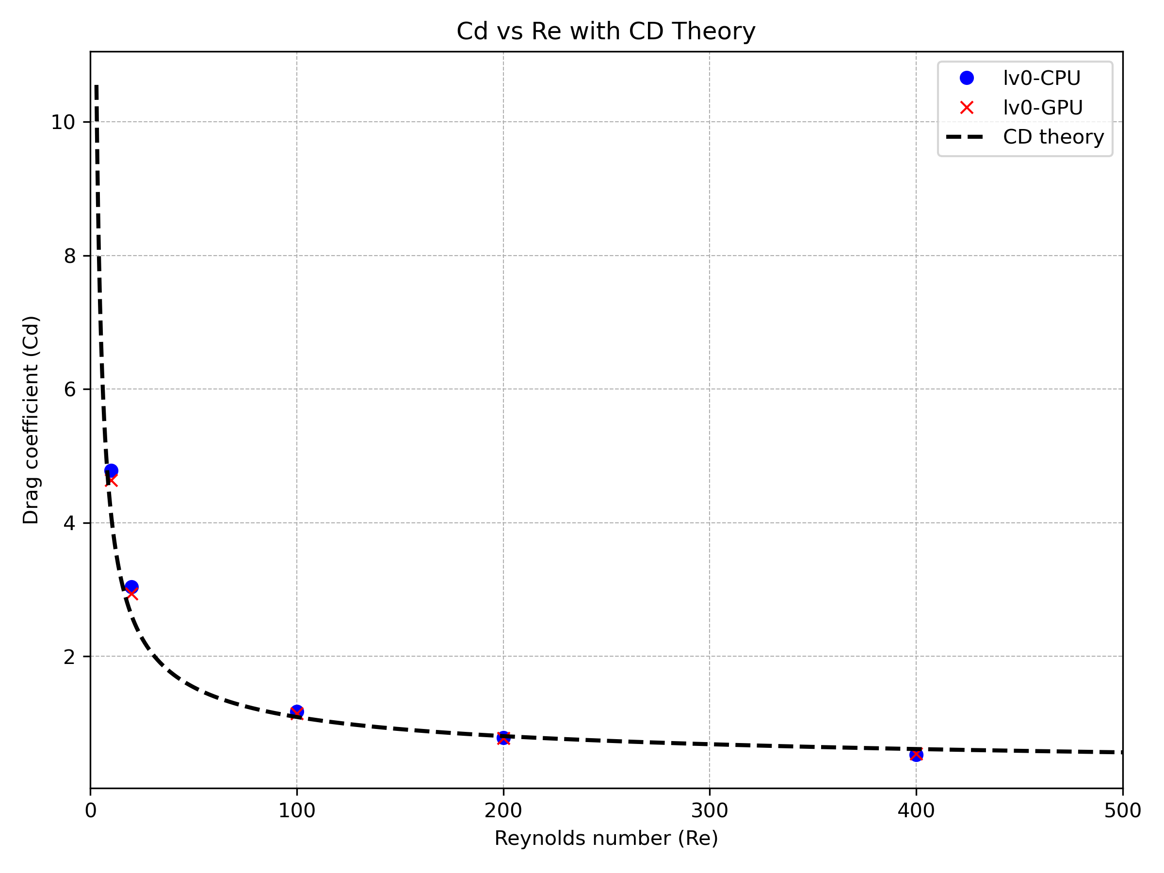
Figure 6 Drag coefficient comparison between CPU and GPU execution modes without adaptive mesh refinement (AMR).
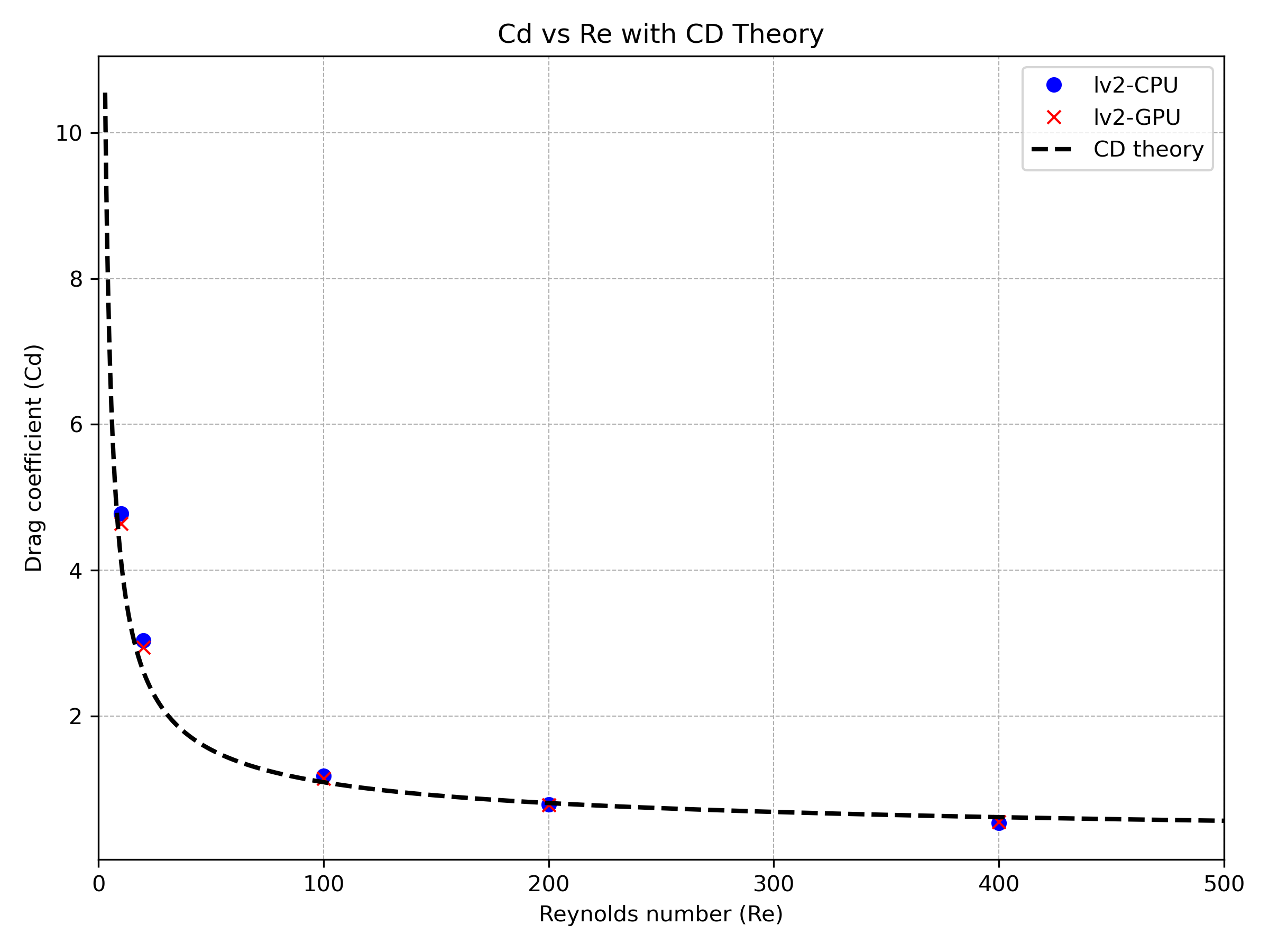
Figure 7 Drag coefficient comparison between CPU and GPU execution modes with adaptive mesh refinement (AMR).
If users encounter discrepancies between CPU and GPU results in any case, please contact us, for example by submitting an issue to the repository.